Splice_sim - Benchmarking RNA-seq mapping in the age of nucleotide Ccnversions
Nucleotide conversion RNA sequencing techniques have revolutionized how we study RNA modifications, stability, and dynamics. From metabolic labeling experiments that track RNA synthesis and decay, to bisulfite sequencing that maps methylation sites - these approaches provide unprecedented insights into post-transcriptional regulation. However, they come with a substantial challenge: the very nucleotide conversions that make these experiments powerful can introduce biases in how reads map to reference genomes.
Our recent paper published in Genome Biology introduces splice_sim, a comprehensive simulation and evaluation framework designed to systematically measure and address these mapping biases. This post will walk you through what the tool does, why it matters, and how you can use it for your own projects.
The Problem: When conversions confuse mappers
Nucleotide conversion (NC) RNA-seq encompasses a broad range of techniques, each introducing specific types of base changes, for instance:
- Metabolic labeling (e.g., SLAM-seq with 4-thiouridine): Introduces T-to-C conversions at low rates (1-5%) to distinguish newly synthesized RNA from pre-existing transcripts
- RNA bisulfite sequencing: Creates C-to-T conversions at very high rates (>98%) to identify methylated cytosines that resist conversion
These mismatches to the reference genome make read mapping more challenging. The question we wanted to address is: how much does this affect our downstream biological interpretations?
Table 1: Overview of Nucleotide Conversion RNA-seq Techniques
| Technique | Conversion Type | Conversion Rate | Key Metric | Biological Application | Example Use Case |
|---|---|---|---|---|---|
| Metabolic Labeling (SLAM-seq, TUC-seq) | T → C | Low (1-5%) | FCR (Fraction Converted Reads) | RNA synthesis, processing, decay kinetics | Measuring RNA half-lives in pulse-chase experiments |
| RNA Bisulfite Sequencing | C → T | Very High (>98%) | metR (Methylation Rate) | Post-transcriptional cytosine methylation (m5C) | Identifying methylated cytosines in cellular transcripts |
| Isoform Analysis (any NC technique) | Variable | Variable | FMAT (Fraction Mature) | Alternative splicing, intron retention | Comparing spliced vs unspliced isoform abundances |
Table 1: Different NC RNA-seq approaches introduce specific types and rates of nucleotide conversions, each with distinct metrics and biological applications. The challenge: all of them introduce mismatches that can bias read mapping.
Consider a metabolic labeling pulse-chase experiment where you’re measuring RNA half-lives. If converted reads (labeled RNA) map with lower accuracy than unconverted reads (unlabeled RNA), your fraction of converted reads (FCR) will be biased, leading to incorrect half-life estimates. For genes involved in critical regulatory pathways, this isn’t just a technical nuisance - it leads to wrong biological conclusions.
Enter splice_sim
Splice_sim is a Python-based simulation and evaluation pipeline that evaluates this problem head-on. It’s built around the core capabilities:
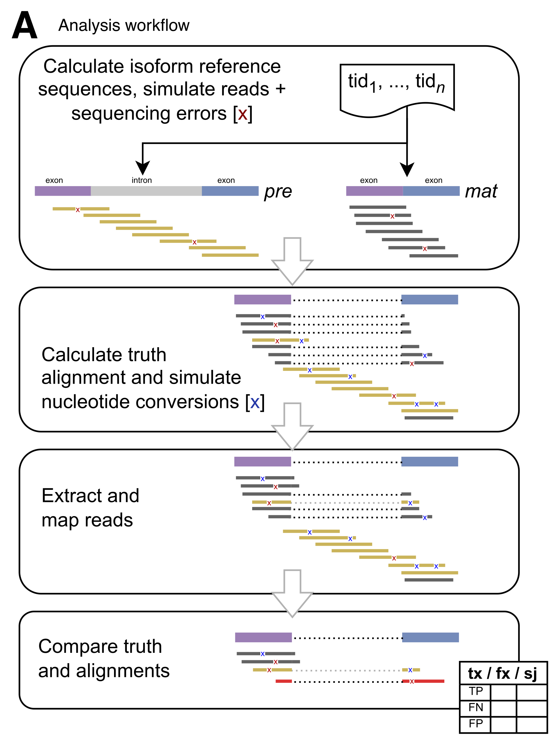
Figure 1: The splice_sim analysis workflow. The pipeline simulates reads with realistic sequencing errors for premature and mature isoforms, injects nucleotide conversions at configured rates, maps reads with evaluated mappers, and compares results to ground truth to calculate TP/FP/FN counts per genomic annotation. (Figure 1A from the paper)
Realistic RNA-seq simulation
The framework simulates RNA-seq reads that mirror real experimental conditions:
- Uses ART for realistic Illumina sequencing errors
- Generates reads from configurable isoform mixtures (premature unspliced and mature spliced transcripts)
- Introduces nucleotide conversions at user-defined rates
- Supports arbitrary single nucleotide variations (SNVs)
Comprehensive Evaluation
Unlike generic mappability scores that operate at the genome-wide level, splice_sim evaluates mapping accuracy for biologically meaningful units:
- Whole transcripts - overall gene-level performance
- Exons and introns - feature-specific accuracy
- Splice junctions - the most challenging mapping scenario
For each annotation, it calculates true positives (TP), false positives (FP), and false negatives (FN), deriving precision, recall, and F1 scores.
Nextflow workflow
The entire pipeline is wrapped in Nextflow workflows with Docker containerization, making it reproducible and easy to deploy across different computing environments - from your laptop to HPC clusters to the cloud.
Key contributions of our study
We used splice_sim to generate deep simulated datasets for mouse and human transcriptomes, evaluating popular splice-aware mappers (STAR and HISAT-3N) under various conversion rates. Here are the headline findings:
Notable metrics 📊 High mappability regions: F1 > 0.98 for both mappers ⚠️ Low mappability regions: F1 < 0.55 - substantial accuracy drop 🧬 Impact on biology: >120 protein-coding genes showed >10% error in half-life estimates 🎯 Mosaic improvement: Reduced outliers from 239 to 95 in half-life analysis 🔬 Methylation sites: 99.2% recall but considerable FP calls in low mappability regions
Mappability dominates, But conversions matter
Mapping accuracies with and without nucleotide conversions were high (F1 > 0.98) for annotations with high or medium genome mappability, but substantially lower (F1 < 0.55) for low mappability regions. This isn’t surprising - repetitive sequences are inherently difficult to map.
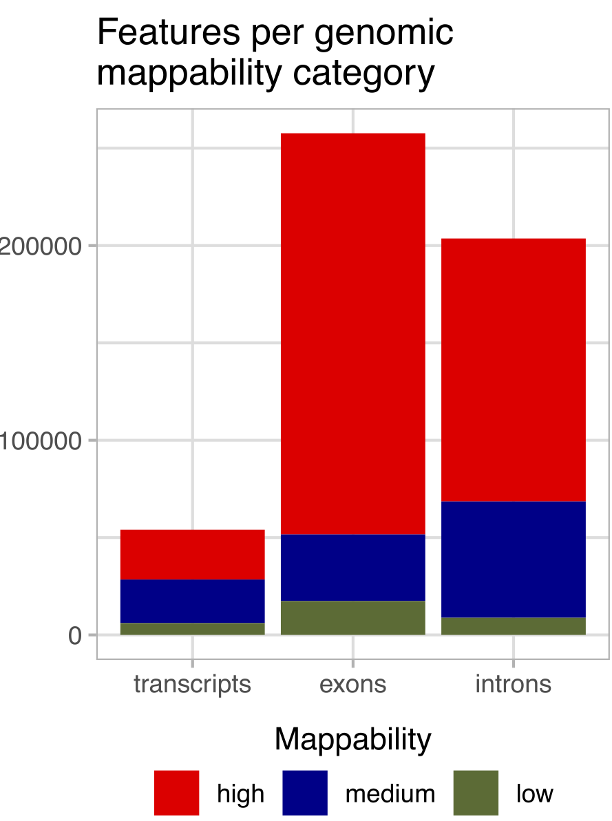
Figure 2: Distribution of analyzed annotations across high (>0.9), medium, and low (<0.2) mean genome mappability categories. Low mappability regions, while smaller in number, are critical for understanding mapping biases. (Figure 1B from the paper)
What does also not come as too big of a surprise is that nucleotide conversion and sequencing errors increased false discovery and false negative rates for both mappers, as read alignment becomes more difficult with increased numbers of mismatches to the originating genomic sequence.
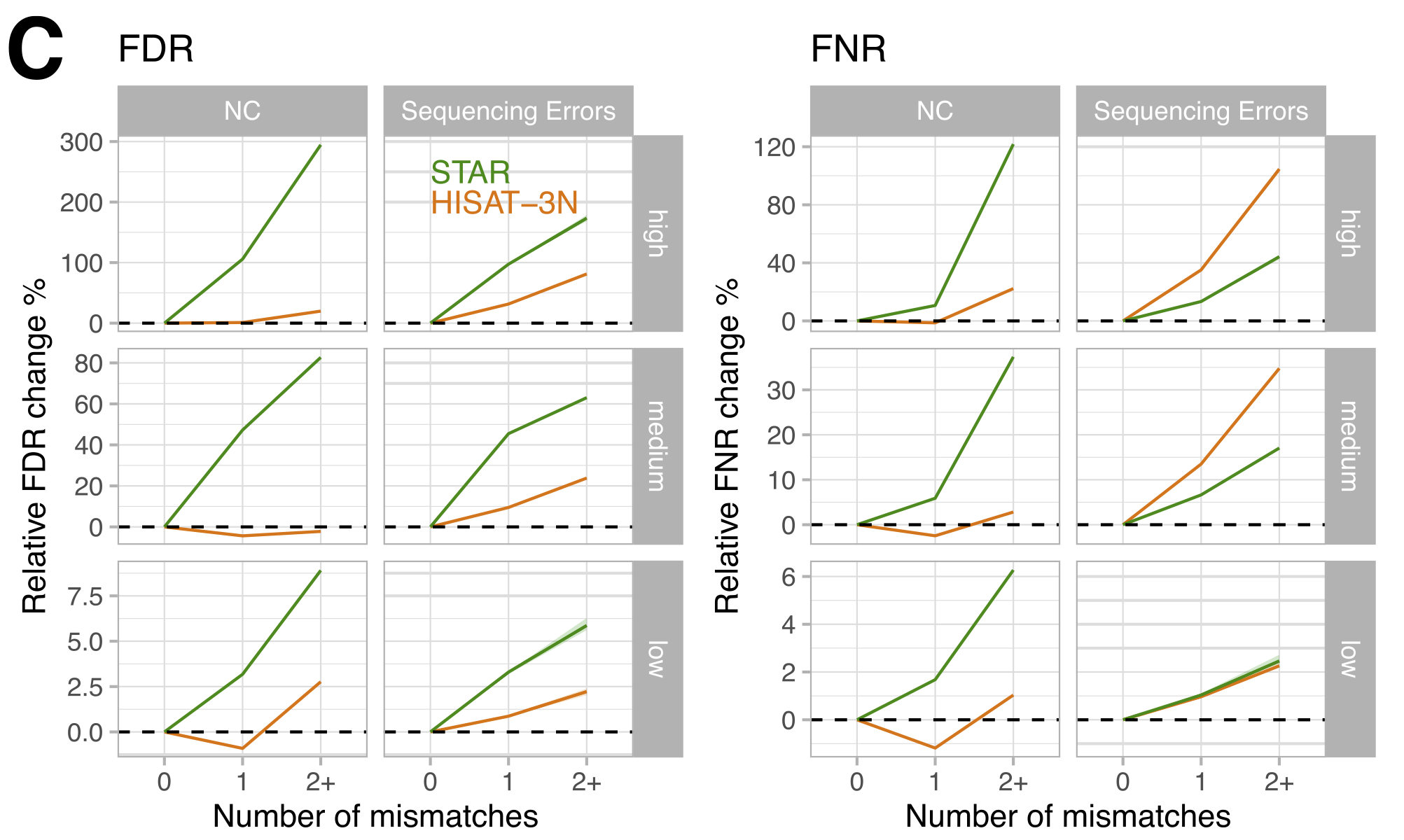
Figure 3: Changes in false discovery (FDR) and false negative rates (FNR) by number of mismatches compared to reads without mismatches, stratified by mappability. Note how HISAT-3N (orange) is largely unaffected by T-to-C conversions due to its 3N mapping approach, while STAR (green) shows increasing error rates with more mismatches. (Figure 1C from the paper)
What is more notable, but somewhat expected is that for STAR, performance degraded with increasing conversion rates. HISAT-3N (a 3-nucleotide mapper that treats T and C as equivalent) was largely unaffected by T-to-C conversions but showed its own quirks, including ~2% of reads mapping to the wrong strand.
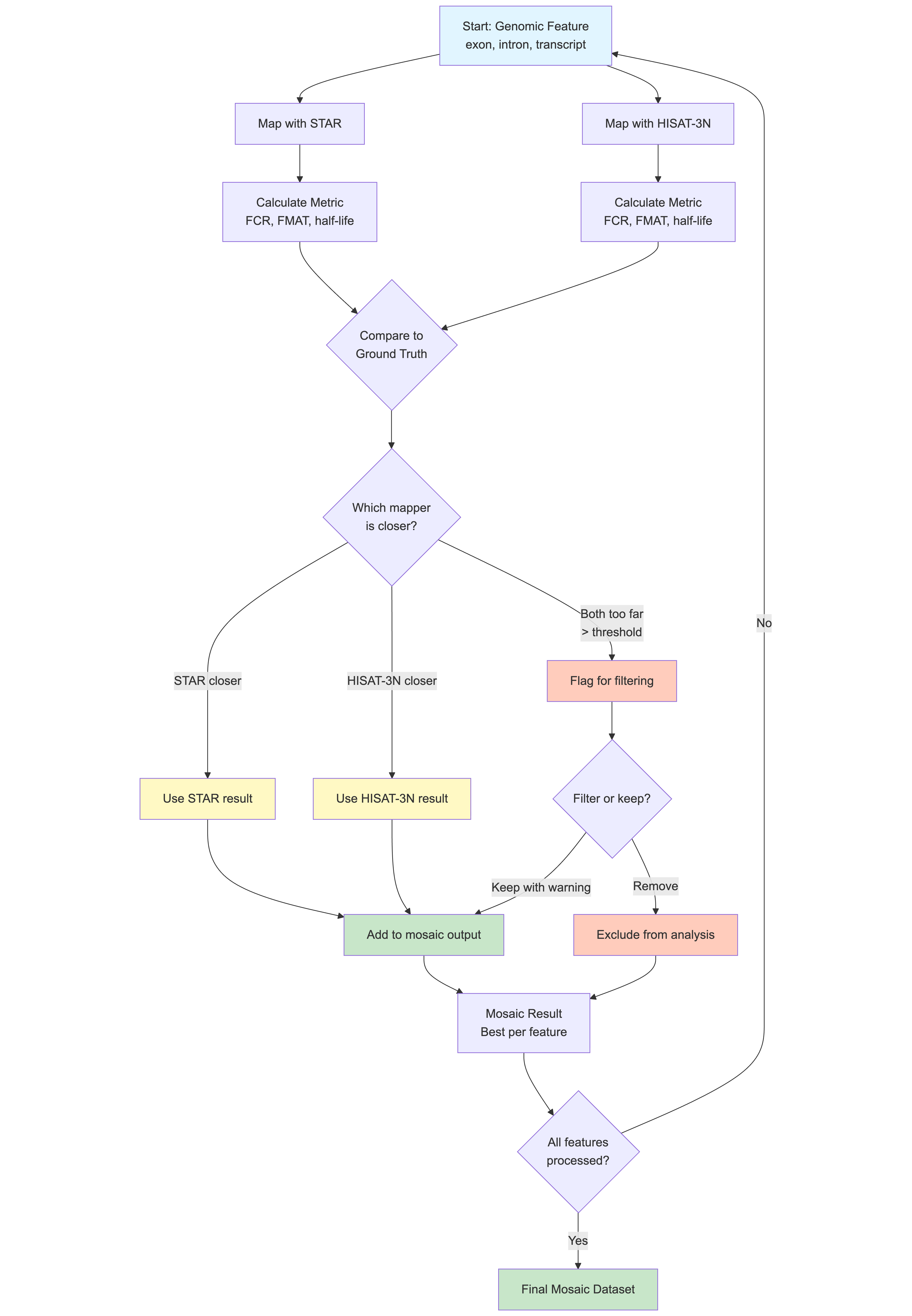
The Mosaic approach: Leveraging mapper strengths
One of the most practical contributions of our study based on the observation that different mappers have different strengths is the “mosaic” analysis strategy. Rather than declaring one mapper superior, we found that different mappers excel in different genomic contexts.
The mosaic approach works like this:
- Map your data with multiple mappers (e.g., STAR and HISAT-3N)
- For each genomic interval, select the result from the mapper with the best accuracy
- Optionally filter intervals where no mapper performs adequately
When combining a mosaic approach with a filtering strategy that removed transcripts for which none of the mappers returned results close to the simulation, the overall mean FCR approached the simulated true value.
This strategy improved FCR reconstruction, reduced half-life outliers, and recovered more accurate FMAT values. It does require running multiple alignments, but the accuracy gains can be substantial for critical analyses.
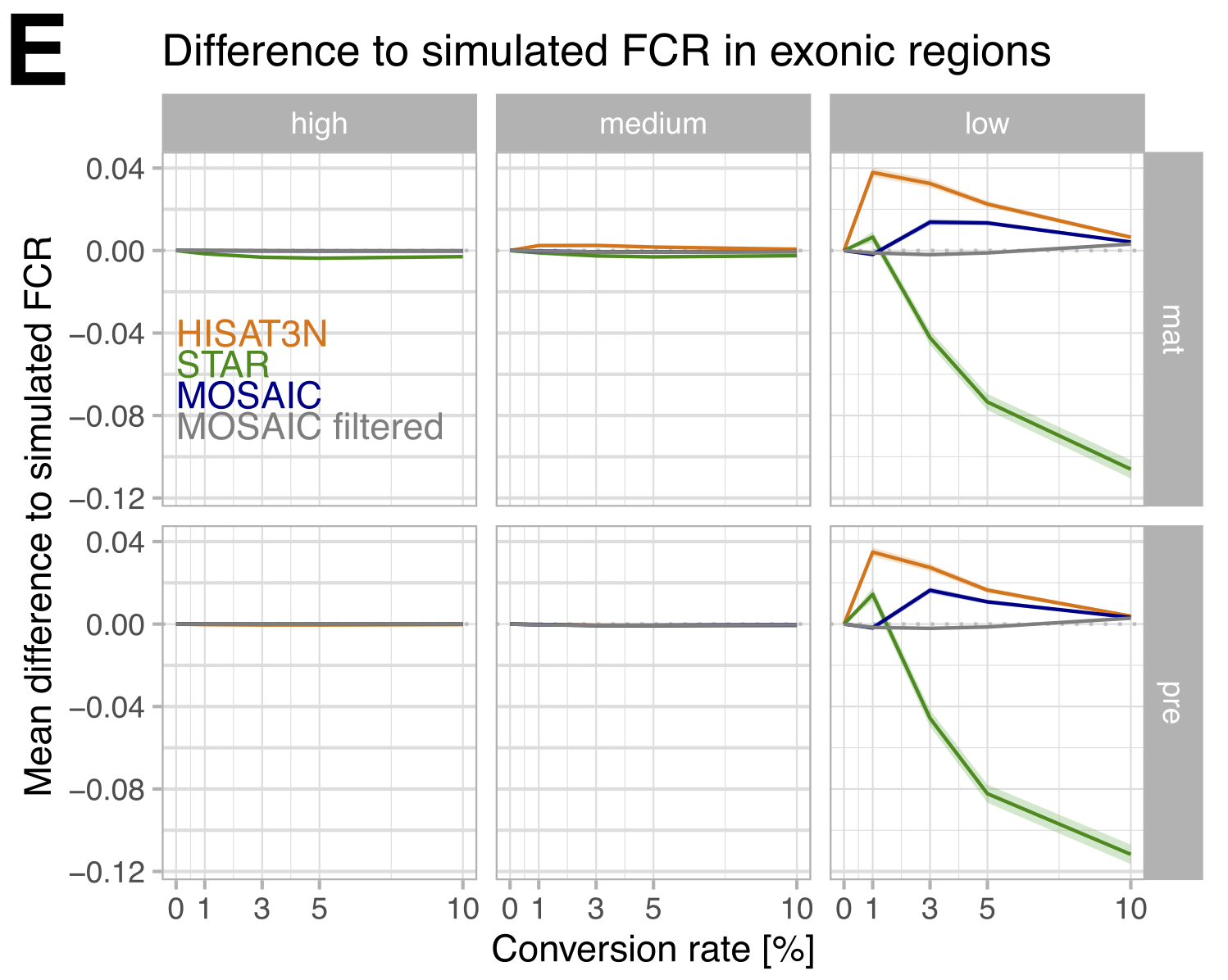
Figure 4: Mean difference to simulated exonic FCR per mapper. The mosaic approach (selecting the best mapper per interval) reduces differences to simulated values, and when combined with filtering, reconstruction is nearly perfect. (Figure 1E from the paper)
Biological consequences: Half-life estimation
We simulated realistic pulse-chase experiments to measure RNA decay rates. Although half-life estimation was robust for most transcripts, a considerable number of outliers showed more than 10% difference to simulated half-lives for both mappers in the medium and low mappability segments. These outliers affected over 120 protein-coding genes - genes that researchers might be studying for their biological relevance.
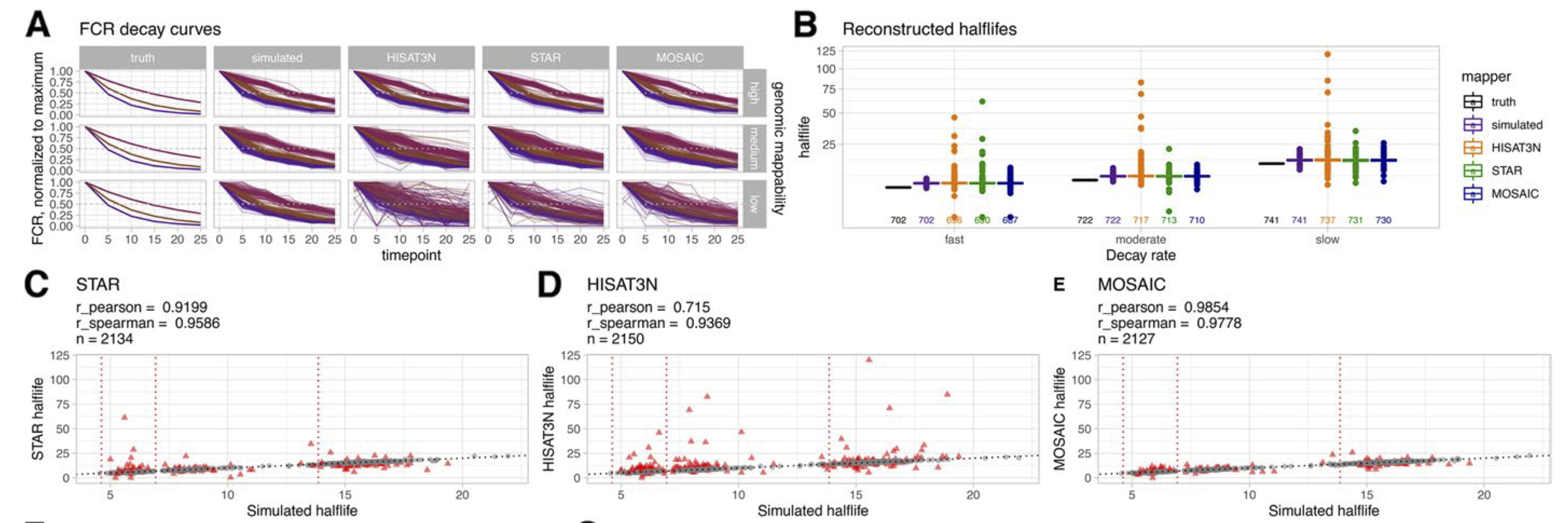
Figure 5: Effect of NC on transcript half-life reconstruction. Top left: Normalized FCR per time point showing increasing noise with decreasing mappability. Top right: Reconstructed half-lives per decay rate. The box plots show a considerable number of outliers for both mappers; numbers of considered transcripts are plotted below the boxes. Bottom: Reconstructed half-lives showing outliers (red triangles) that deviate >10% from simulated values. The mosaic approach (bottom) combining both mappers reduces outliers considerably. (Figure 2 from the paper)
Isoform quantification challenges
Alignment of spliced reads is particularly difficult as it needs to take the possibility of large gaps due to spliced out introns into account and requires accurate placement of short sub-sequences of reads (anchors) that span over these gaps.
We found that transcripts often contain a mosaic of high, medium, and low mappability introns. By implementing an intron filtering strategy that removes problematic introns, we improved the accuracy of mature isoform fraction (FMAT) estimates considerably.
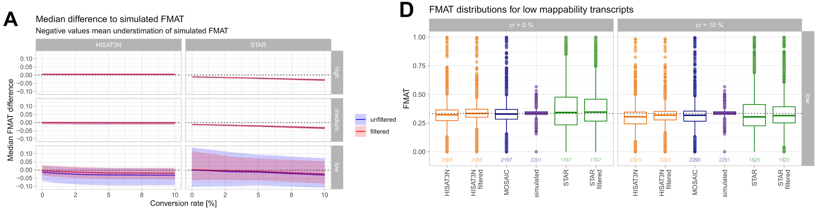
Figure 6: FMAT (fraction of mature isoform) reconstruction improves with intron filtering. Left: Median difference to simulated FMAT showing improvement with filtering (solid vs dashed lines). Right: Distribution of FMAT values for low mappability transcripts shows that both filtering and the mosaic approach recover more accurate estimates closer to the theoretical value of 1/3. (Figure 3A and 3D from the paper)
Methylation site calling hotspots
For RNA bisulfite sequencing analysis, low mappability regions are hotspots of false cytosine methylation calls. All mappers produced considerable amounts of false positive and a few false negative m5C calls, mainly in low mappability regions of protein coding genes.
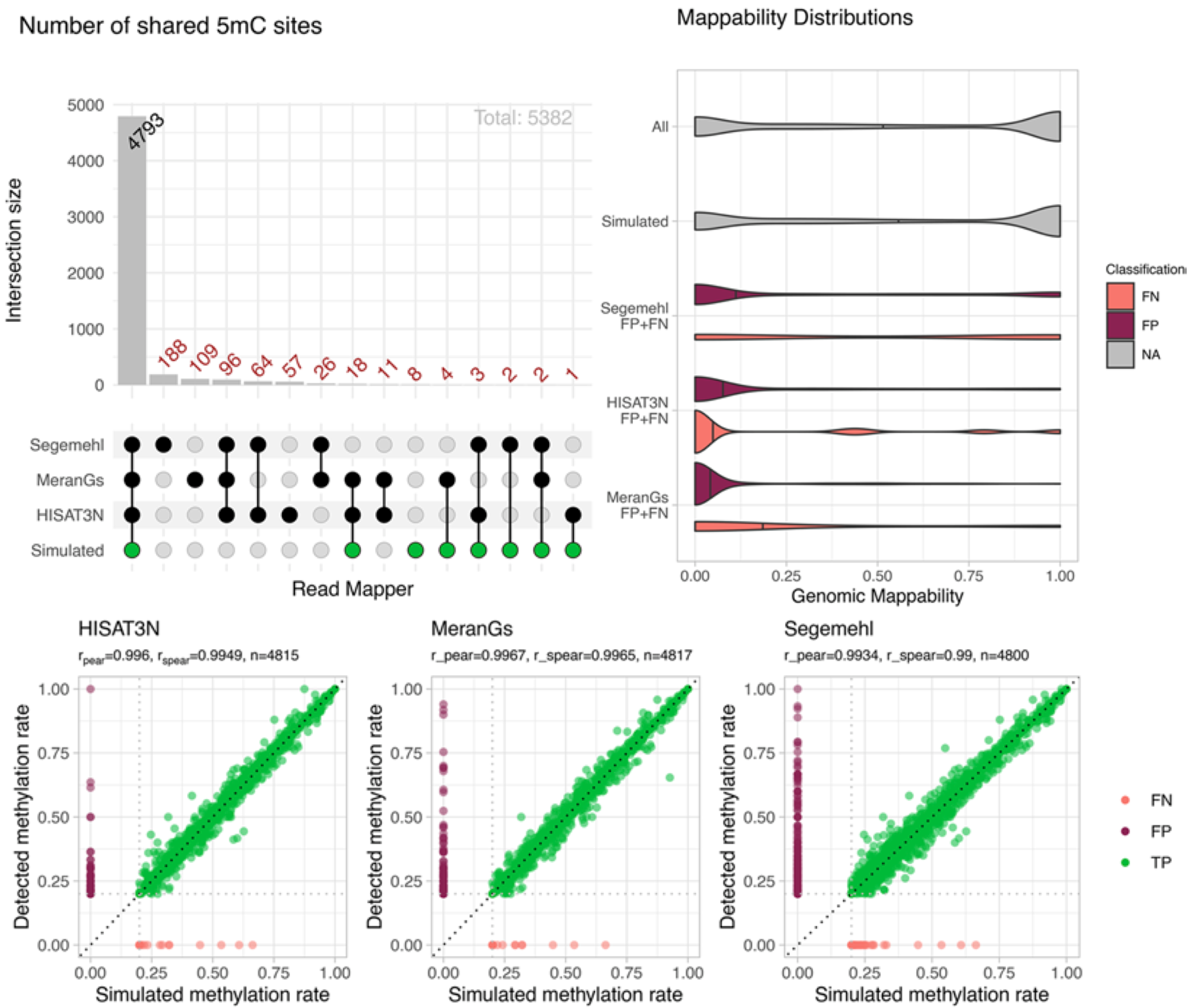
Figure 7: Effect of mappability on methylation site reconstruction. Most m5C sites were recovered correctly, but false positives (FP) and false negatives (FN) were predominantly located in low mappability regions. The correlation plots show methylation rates for HISAT-3N, meRanGs, and Segemehl with TP calls in green and false calls in red. (Figure 4 from the paper)
This has important implications for establishing accurate m5C site catalogs, which have varied wildly in the literature (from <100 to >10,000 sites reported).
Pre-computed mapping accuracy tables: Ready-to-use resources
One of the most immediately useful outputs from our study is a comprehensive set of pre-computed mapping accuracy tables for mouse (mm10) and human (GRCh38) transcriptomes, covering over 50,000 transcripts each. These tables are freely available on Zenodo and provide detailed performance metrics for every annotated transcript, exon, intron, and splice junction.
What’s included in these tables:
- Mapping accuracy scores (F1, precision, recall) for STAR and HISAT-3N across different conversion rates (0%, 1%, 3%, 5%, 10%)
- Mappability classifications (high, medium, low) for each genomic feature
- FCR and FMAT reconstruction accuracy per feature
- Recommendations for which mapper performs best for each transcript
How to use them:
- Before starting an experiment: Look up your genes of interest to assess whether they have sufficient mappability for reliable NC RNA-seq analysis
- During data analysis: Filter out problematic transcripts/introns with known mapping issues
- Choosing a mapper: Select the optimal mapper (or apply the mosaic strategy) based on pre-computed performance for your specific genes
- Quality control: Flag results from low-accuracy regions for additional validation
📊 Ready-to-Use Data
- Mouse (mm10): >50,000 GENCODE transcripts evaluated
- Human (GRCh38): >50,000 Ensembl canonical transcripts evaluated
- Conditions tested: 0%, 1%, 3%, 5%, 10% T-to-C conversion rates
- Mappers evaluated: STAR, HISAT-3N (metabolic labeling) + meRanGs, Segemehl (BS-seq)
- Format: TSV.gz tables ready to import into R or Python
Available at: https://doi.org/10.5281/zenodo.11196570
Beyond mouse and human:
The beauty of splice_sim is that it’s not limited to these two species. The framework is designed to work with any genome and annotation set. Want to evaluate NC mapping accuracy for:
- Zebrafish developmental studies?
- Drosophila genetics experiments?
- Arabidopsis plant biology?
- Yeast time-course experiments?
- Non-model organisms with custom annotations?
Simply provide your reference genome FASTA, gene annotation GFF3, and run splice_sim with your experimental parameters. The pipeline will generate the same comprehensive mapping accuracy tables tailored to your organism and genes of interest.
This is particularly valuable for researchers working on:
- Organisms with less well-characterized repetitive elements
- Custom or alternative gene annotations
- Novel transcripts or isoforms not in standard databases
- Organisms with different genome complexity and mappability landscapes
The paper provides detailed protocols and configuration examples for running splice_sim on arbitrary species, making it a truly universal tool for the NC RNA-seq community.
Practical applications: What can you do with splice_sim?
1. Pre-experiment planning
Before committing to expensive sequencing, simulate your experimental design:
# Configure your experiment in JSON
{
  "condition": {
    "ref": "T",
    "alt": "C",
    "conversion_rates": [0.01, 0.03, 0.05],
    "base_coverage": 50
  },
  "transcript_ids": "genes_of_interest.tsv"
}

# Run the simulation
nextflow run splice_sim.nf -profile docker -c my_config.json
This tells you whether your genes of interest have sufficient mappability for reliable analysis, or if you need to adjust your approach (longer reads, different protocol, etc.).
2. Benchmark your pipeline
Evaluating a new mapper or tweaking parameters? Run it against splice_sim-generated ground truth data:
# Add your custom mapper to the config
"mappers": {
  "MY_MAPPER": {
    "cmd": "my_mapper",
    "index": "/path/to/index",
    "options": "--custom-parameters"
  }
}
The evaluation module will give you detailed per-feature accuracy metrics.
3. Data quality control
Use our pre-computed mapping accuracy tables for mouse and human transcriptomes (available on Zenodo) to:
- Filter transcripts/exons/introns with poor mapping accuracy
- Identify which mapper works best for your genes of interest
- Apply targeted filtering strategies to improve downstream analyses
4. Comparing sequencing strategies
We used splice_sim to compare full-transcript sequencing versus 3’ end sequencing. While simulated 3’ end sequencing data showed higher mapping accuracies across all conversion rates and mappability classes due to higher mappability, full-length sequencing showed the smallest deviation from the simulated FCR, implying that the larger mapping space of the full transcript allows for more robust FCR estimates.
You can set up similar comparisons for your specific use case.
Getting started with splice_sim
The tool is available on GitHub with comprehensive documentation. Here’s a quick-start guide:
Installation
The easiest way is via Docker - all dependencies are pre-packaged:
# Pull the Docker image
docker pull tobneu/splice_sim:release

# Or for HPC environments with Singularity
singularity pull docker://tobneu/splice_sim:release
For local development, create a conda environment:
conda env create -f environment.yml
conda activate splice_sim
Running a simple simulation
The framework uses a central JSON configuration file to define all parameters. Here’s a minimal example for a small test:
{
  "dataset_name": "my_test_run",
  "splice_sim_cmd": "python /path/to/splice_sim/main.py",
  "gene_gff": "/references/gencode.vM21.gff3.gz",
  "genome_fa": "/references/mm10.fa",
  "genome_chromosome_sizes": "/references/mm10.chrom.sizes",
  "transcript_ids": "test_genes.tsv",
  "isoform_mode": "1:1",
  "condition": {
    "ref": "T",
    "alt": "C",
    "conversion_rates": [0.02, 0.05],
    "base_coverage": 50
  },
  "mappers": {
    "STAR": {
      "star_cmd": "STAR",
      "star_genome_idx": "/indices/star_index",
      "star_splice_gtf": "/references/genes.gtf"
    }
  },
  "readlen": 100,
  "random_seed": 42
}
Run the complete workflow:
# Simulation workflow
nextflow run splice_sim.nf -c my_config.json -profile docker

# Evaluation workflow
nextflow run splice_sim_eva.nf -c my_config.json -profile docker
Understanding the output
Splice_sim generates several types of output:
Count tables (count/*.counts.tsv.gz): Raw TP/FP/FN counts per mapper, conversion rate, and genomic feature
Metadata tables (meta/*.metadata.tsv.gz): Feature characteristics including mappability, GC content, convertibility
Performance metrics: Precision, recall, and F1 scores calculated from count tables
Visual tracks: Optional TDF files for viewing in IGV, highlighting misaligned reads
Output directory structure
results/
├── simulation/
│   ├── model/
│   │   ├── transcript_model.pkl          # Transcript isoform definitions
│   │   ├── sequences.fa                  # Simulated transcript sequences
│   │   └── model_config.json             # Model parameters
│   │
│   ├── reads/
│   │   ├── condition_0pct/               # Unconverted reads
│   │   │   ├── simulated_reads.fq.gz
│   │   │   └── truth_alignments.bam
│   │   ├── condition_2pct/               # 2% conversion rate
│   │   │   ├── simulated_reads.fq.gz
│   │   │   └── truth_alignments.bam
│   │   └── condition_5pct/               # 5% conversion rate
│   │       ├── simulated_reads.fq.gz
│   │       └── truth_alignments.bam
│   │
│   └── alignments/
│       ├── STAR/
│       │   ├── condition_0pct.bam
│       │   ├── condition_2pct.bam
│       │   └── condition_5pct.bam
│       └── HISAT3N/
│           ├── condition_0pct.bam
│           ├── condition_2pct.bam
│           └── condition_5pct.bam
│
├── evaluation/
│   ├── count/
│   │   ├── STAR_0pct_tx.counts.tsv.gz    # Transcript-level counts
│   │   ├── STAR_0pct_fx.counts.tsv.gz    # Exon/intron counts
│   │   ├── STAR_0pct_sj.counts.tsv.gz    # Splice junction counts
│   │   ├── HISAT3N_0pct_tx.counts.tsv.gz
│   │   └── ...
│   │
│   ├── meta/
│   │   ├── tx.metadata.tsv.gz            # Transcript metadata
│   │   ├── fx.metadata.tsv.gz            # Exon/intron metadata
│   │   └── sj.metadata.tsv.gz            # Splice junction metadata
│   │
│   ├── tracks/                            # Optional IGV visualization
│   │   ├── STAR_0pct_FP.tdf              # False positive tracks
│   │   ├── STAR_0pct_FN.tdf              # False negative tracks
│   │   └── ...
│   │
│   └── processed/
│       ├── combined_results.rds           # R data object
│       └── summary_stats.tsv              # Summary statistics
│
├── reports/
│   ├── execution_report.html              # Nextflow execution report
│   ├── timeline.html                      # Pipeline timeline
│   └── trace.txt                          # Resource usage
│
└── logs/
    ├── simulation.log
    ├── mapping.log
    └── evaluation.log
Key files to focus on:
count/*.counts.tsv.gz- TP/FP/FN counts for calculating accuracy metricsmeta/*.metadata.tsv.gz- Mappability, GC content, and other feature characteristicsprocessed/combined_results.rds- Pre-processed data ready for analysis in Rtracks/*.tdf- Visual tracks for exploring specific mapping errors in IGV
The evaluation results can be imported into R for detailed analysis using the provided preprocessing script:
Rscript splice_sim/src/main/R/splice_sim/preprocess_results.R \
  my_config.json output_dir/
Advanced use cases
Custom nucleotide conversion models
While splice_sim uses Bernoulli processes for NC simulation (appropriate for BS-seq and SLAM-seq), you might need more sophisticated models. For example, A-to-I RNA editing by ADAR enzymes shows sequence-context dependencies.
The NC simulation is implemented as a Python method with access to:
- Read sequence (without NC)
- Genomic coordinates and strand
- Configured reference/alternate bases
- Conversion rate
- List of convertible positions
- Any configured SNPs
Simply modify the splice_sim.simulator.modify_bases method to implement your custom conversion logic.
Paired-end support
The current version focuses on single-end reads, which are cost-effective for many experiments. However, paired-end data offers advantages:
- Improved mappability from both mates
- Error correction in overlapping regions
Paired-end support is on the TODO list.
Integrating with AWS batch
Since splice_sim uses Nextflow, you can easily scale to cloud computing. Here’s a basic AWS Batch configuration:
profiles {
    awsbatch {
        process.executor = 'awsbatch'
        process.queue = 'my-batch-queue'
        process.container = 'tobneu/splice_sim:release'
        workDir = 's3://my-bucket/work'
    }
}
This is particularly useful when simulating large datasets (full transcriptomes) or evaluating multiple mappers across many parameter combinations.
Recommended best practices
Based on our findings, here are practical recommendations for NC RNA-seq analysis:
For metabolic labeling experiments
- Always check mappability: Use our pre-computed tables or run splice_sim on your genes of interest
- Consider a mosaic approach: If computationally feasible, map with both STAR and HISAT-3N and combine results
- Filter carefully: Remove low-mappability transcripts or apply targeted filtering strategies
- Validate biological findings: If a half-life estimate seems suspicious, check the mappability and conversion rate dependency
For RNA bisulfite sequencing
- Use specialized mappers: HISAT-3N, meRanGs, or Segemehl perform better than standard mappers
- Be extra cautious with low mappability regions: These are hotspots for false m5C calls
- Cross-validate calls: Don’t rely solely on methylation rates for filtering - consider mappability and structural context
- Expect protocol artifacts: Incomplete conversion and missing reads in low mappability regions are inherent to the protocol
For isoform analysis
- Provide known splice sites: This dramatically improves spliced read mapping accuracy
- Filter problematic introns: Use splice_sim’s approach to remove introns with poor FMAT reconstruction
- Check for intron mappability mosaics: Transcripts often mix high and low mappability introns
- Validate novel splice junctions carefully: False-positive SJ calls increase with conversion rates
Limitations and future directions
While splice_sim is powerful, it has some limitations worth noting:
Simulation-based: Results depend on stochastic processes, though our replicate analysis showed high correlation
Worst-case FP scenarios: Our main dataset simulates equal coverage for all transcripts, potentially inflating false positives. For your cell type, configure transcript abundances from real RNA-seq data.
Single-end only: Currently limited to single-end reads, though paired-end support is planned
Bernoulli NC model: May not capture sequence-context dependencies in some NC types
Despite these limitations, splice_sim provides an invaluable framework for understanding and mitigating NC mapping biases.
Conclusion
Nucleotide conversion RNA-seq techniques provide powerful insights into RNA biology, but their mapping biases can lead to substantial errors in biological interpretation. Splice_sim offers both a diagnostic tool to understand these biases and practical strategies to mitigate them.
The framework is:
- Comprehensive: Evaluates mapping accuracy at multiple biologically meaningful scales
- Flexible: Configurable for diverse experimental designs and organisms
- Actionable: Provides concrete strategies (mosaic approach, filtering) to improve analysis
- Accessible: Wrapped in Nextflow with Docker containerization for easy deployment
Whether you’re planning a new NC RNA-seq experiment, benchmarking analysis pipelines, or trying to understand unexpected results from existing data, splice_sim can help ensure your biological conclusions rest on solid computational ground.
Resources
- Paper: Genome Biology publication
- Source Code: GitHub repository
- Docker Image: Docker Hub
- Precomputed Data: Zenodo repository with mapping accuracy tables for mouse and human
Have questions or want to discuss NC RNA-seq mapping challenges? Feel free to open an issue on GitHub or reach out directly. Happy simulating!