Orbital basics

I was always fascinated by rockets, space in general and zero-gravity environments, however the Math’s involved always deemed too complex for me. However, through the playful and still complex approach of Kerbal Space Program (KSP) - it is an awesome game I totally recommend to anybody remotely interested in space exploration - I picked up interest lately again and started reading into orbital mechanics, propulsion systems and related stuff in more detail.

This blog series is dedicated to summarising basic concepts at definitely super simplified and probably sometimes oversimplified and not entirely correct level.

The easiest concept for me to grasp, since once can do it quite interactively in KSP is the concept of orbits and orbital changes through orbital maneuvers.

So this very first post of this series will cover my basic understanding of the concept of orbits.

Ellipse

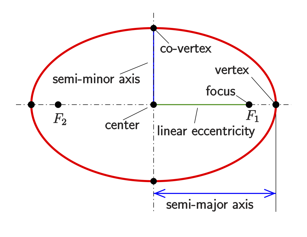
Let’s start of with refreshing our memory what an ellipse is - because that is what most relevant orbits for this blog series will look like. In mathematical terms, an ellipse is a plane curve surrounding two focal points (\(F_1\) and \(F_2\)), such that for all points on the curve, the sum of the two distances \(d(F_1) + d(F_2)\) is constant.

It is a generalization of a circle, where the two focal points are the same. Yes, also circular orbits exist.

Ellipse parameters

There are a few important parameters describing an ellipse which will be referred throughout this blog series, so make sure you memorize and understand them, because they will keep popping up again and again.

Semi-major and semi-minor axes \(a \geq b\)

\(a\) is referred to as the semi-major axis, i.e. \(a \geq b > 0\).

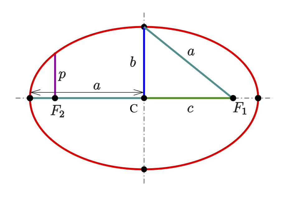
Linear eccentricity \(c\)

This is the distance from the center to any of the two foci: \(c = \sqrt{a^2 - b^2}\).

Eccentricity \(e\)

The eccentricity is expressed as:

\[e = \frac{c}{a} = \sqrt{1 - (\frac{b}{a})^{2}}\]

assuming \(a > b\). An ellipse with equal axes \((a = b)\) has zero eccentricity and is a circle.

Semi-latus rectum \(l\)

The length of the chord through one of the foci, perpendicular to the major axis, is called the latus rectum. One half of it is the semi-latus rectum \(l\). A calculation shows:

\[l = \frac{b^2}{a} = a(1-e^2)\]

The semi-latus rectum \(l\) is equal to the radius of curvature of the osculating circles at the vertices.

Orbit

Now probably everybody has some idea what an orbit is, but before going into details, let’s first summarise the definitions I found on the web.

Definition

In physics, an orbit is the gravitationally curved trajectory of an object, like the the trajectory of any plane around a star or a satellite around earth. Unless mentioned differently, in this blogpost orbit refers to a regularly repeating trajectory, but there are also non-repeating trajectories. To a close approximation, planets and satellites follow elliptic orbits, with the central mass being orbited at on of the two focal points of the ellipse, as described by Kepler’s laws of planetary motion.

The post will stick to the classical Newtonian mechanics paradigm of describing orbital motion, which is an adequate approximation for most situations. However, Einstein’s generaly theory of relativity, which accounts for gravity as due to curvature of spacetime and orbits following geodesics, provides a more accurate calculation and understanding of the exact mechanics of orbital motion, which is needed in near very massive bodies (e.g. Mercury’s orbit around the sun) or for extreme precision (as for GPS satellites).

Understanding orbits

There are two factors involved for understanding orbits:

• Gravity pulling an object from its straight path into a curved path
• The velocity at which this object is trying to travel along its path

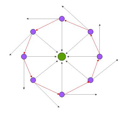
This principal is illustrated by the illustration above, where gravity from a massive body in the center (green) pulls a object travelling on a straight path (pink object, black arrows), effectively bending the path with its constant pull (red) around the center body.

Another way how to illustrate how orbits develop is the though experiment of Newton’s cannonball. Here, we visualize a cannon on top of a very high mountain which can fire at any imaginable speed.

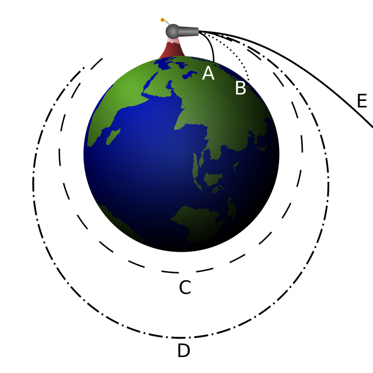
If the cannon fires its ball with a low initial speed, the trajectory of the ball curves downward and hits the ground (A). As the firing speed is increased, the cannonball hits the ground farther (B) away from the cannon, because while the ball is still falling towards the ground, the ground is increasingly curving away from it (see first point, above). All these motions are actually “orbits” in a technical sense – they are describing a portion of an elliptical path around the center of gravity – but the orbits are interrupted by striking the Earth. The horizontal speed for both (A) and (B) is 0 - 7,000 m/s for Earth.

If the cannonball is fired with sufficient speed, the ground curves away from the ball at least as much as the ball falls – so the ball never strikes the ground. It is now in what could be called a non-interrupted, or circumnavigating, orbit. For any specific combination of height above the center of gravity and mass of the planet, there is one specific firing speed (unaffected by the mass of the ball, which is assumed to be very small relative to the Earth’s mass) that produces a circular orbit, as shown in (C).

As the firing speed is increased beyond this, non-interrupted elliptic orbits are produced; one is shown in (D). If the initial firing is above the surface of the Earth as shown, there will also be non-interrupted elliptical orbits at slower firing speed; these will come closest to the Earth at the point half an orbit beyond, and directly opposite the firing point, below the circular orbit. The horizontal speed for both (C) and (D) ranges from 7,300 to 10,000 m/s for Earth.

At a specific horizontal firing speed called escape velocity, dependent on the mass of the planet, an open orbit (E) is achieved that has a parabolic path. At even greater speeds the object will follow a range of hyperbolic trajectories. In a practical sense, both of these trajectory types mean the object is “breaking free” of the planet’s gravity, and “going off into space” never to return. This involves any horizontal speed > 10,000 m/s for Earth.

Various firing speeds of Newton’s cannon and the resulting trajectory.

This leads to four practical classes of moving objects:

1. No orbit

2. Suborbital trajectories

   • Range of interrupted elliptical paths

3. Orbital trajectories

   • Range of elliptical paths with closes point opposite firing point
   • Circular path
   • Range of elliptical paths with closes point at firing point

4. Open (escape) trajectories

   • Parabolic paths
   • Hyperbolic paths

Apsis

The first two terms I learned about in KSP were the two apsis - probably because a lot of orbital maneuvers happen at those and they are pretty simple to comprehend.

Apsis denotes either of the two extreme points (i.e., the farthest or nearest point) in the orbit of a planetary body about its primary body.

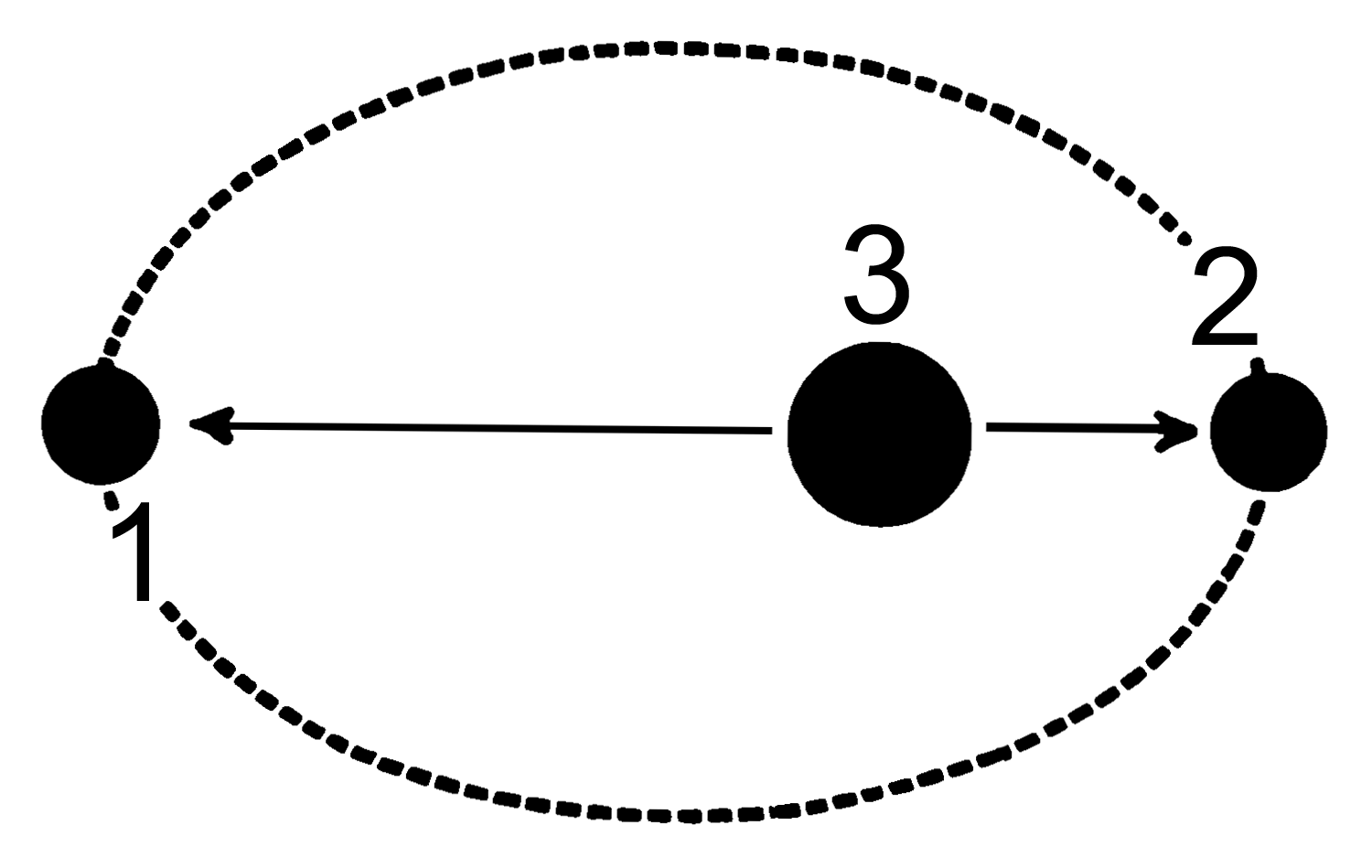
There are two apsides in any elliptic orbit. Each is named by selecting the appropriate prefix: apo- , or peri- and then joining it to the reference suffix of the “host” body being orbited. The general form is apoapsis (see figure above (1)) for the farthest point and periapsis (see top figure (2)) for the nearest point. Depending what central body is orbited it will become apogee and perigee for object orbiting earth, apohelion and perihelion for objects orbiting the sun etc.

Orbital elements

Orbital elements are the parameters required to uniquely identify a specific orbits. In celestial mechanices, usually a Kepler orbit is used. A real orbit changes over time due to gravitational perturbations by other objects and relativistic effects, so a Keplerian orbit is merely an idealized, mathematical approximation at a particular time.

An orbit is generally defined by six elements (known as Keplerian elements) that can be computed from position and velocity:

Two define the size and shape of the trajectory (compare with ellipse parameters):

• Semimajor axis \(a\)

• Eccentricity \(e\)

Two elements define the orientation of the orbital plane in which the ellipse is embedded:

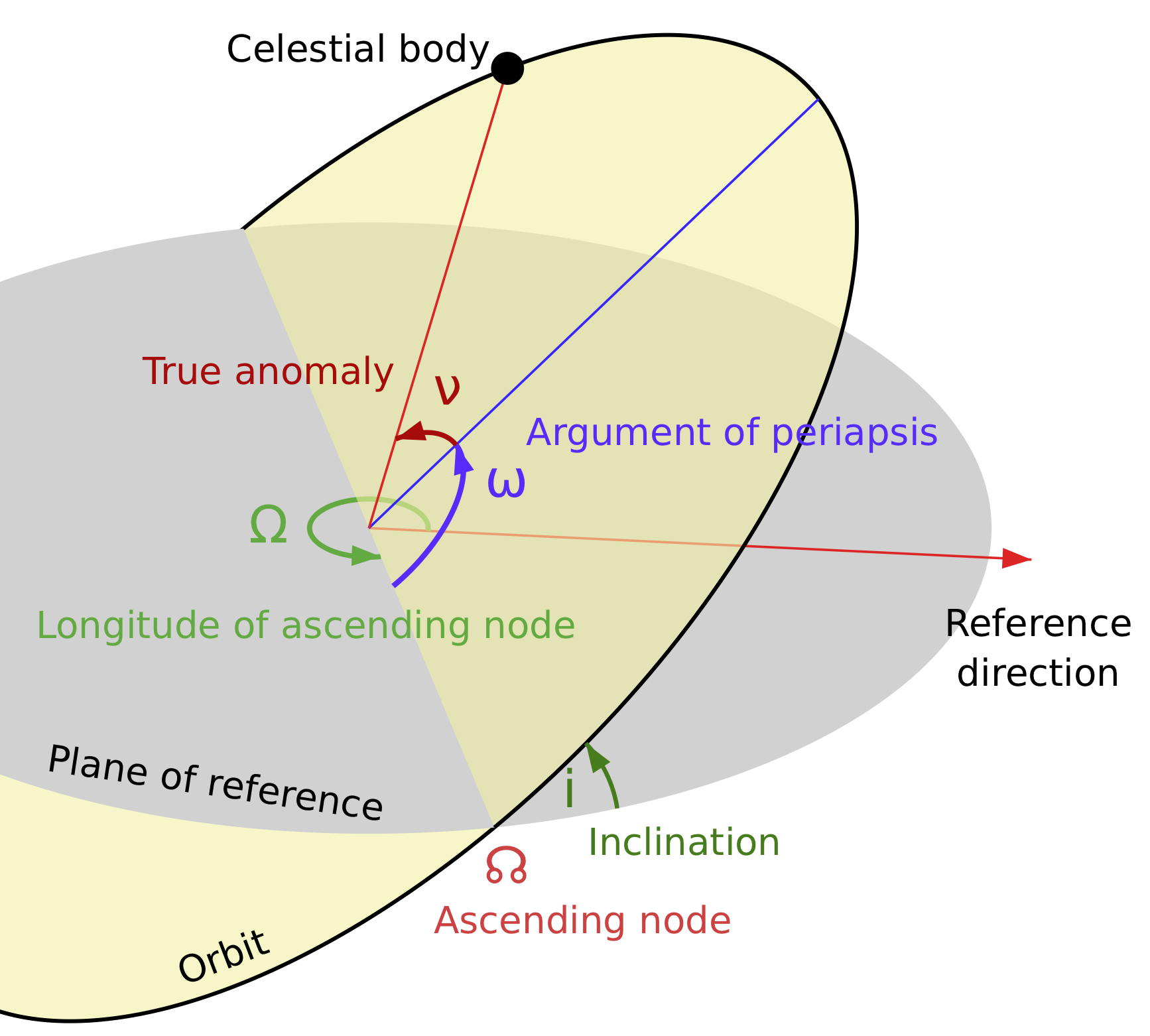
• Inclination \(i\) - vertical tilt of the ellipse with respect to the reference plane (for the earth e.g. the equatorial plane), measured at the ascending node. The ascending node is where the orbit passes upwards through the reference plane). The tilt angle is measured perpendicular to the line of intersection between the orbital plane and the reference plane.

• Longitude of the ascending node \(\Omega\) - horizontally orients the ascending node of the ellipse with respect to the reference frame’s vernal point .

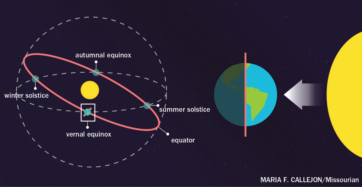
I found it pretty hard at first to wrap my head around what the vernal point actually is - naturally it is some arbitrary reference point to fix the angle for the ascending node \(\Omega\). So actually the vernal point is one of the equinoctes, namely the one occurring in spring in the northern hemisphere. It is regarded as the instant of time when the plane of the Earth’s equator passes through the center of the sun. So at the equator, the sunrays will hit the earth perpendicular directly from the sky zenith. After passing the vernal point, the northern hemisphere will receive more light - summer is here - before the vernal point, the northern hemisphere received less light - winter was coming. Same is true vice versa for the southern hemisphere.

The two remaining elements are as follows:

• Argument of periapsis \(\omega\) defines the orientation of the ellipse in the orbital plane. It is measured as the angle from the ascending node to the periapsis.

• True anomaly (\(v\), \(\theta\), or \(f\)) at epoch (\(M_0\)) defines the position of the orbiting body along the ellipse at a specific time (“epoch”). The true anomaly is an angular parameter defining the angle between the direction of the periapsis and the current position of the orbiting body.

Epoch sounds pretty sophisticated, but basically just just a moment in time used as a reference point for some time-varying astronomical quantity, like the true anomaly. Still sounds complicated?

Let’s look at some unit indicating a specific epoch: J2000.

The \(J\) unit refers to Julian years, which are intervals with the length of a mean year in the Julian calendar, i.e. 365.25 days. This interval measure does not itself define any epoch: the Gregorian calendar is in general use for dating. Thus “J2000” refers to the instant of 12:00 TT (noon) on January 1, 2000.

Now an arbitrary Julian epoch is therefore related to the Julian date by

\[J = 2000 + (Julian date − 2451545.0) ÷ 365.25\]

So in a sense everybody has definitely a feeling for an Epoch because we also structure our lifes and set up meetings for certain “Epochs” everyday.

Orbital period

The orbital period is simply how long an orbiting body takes to complete one orbit.

Ellipse vs orbits

For elliptical orbits, some formulas from ellipses are directly related.

Let \(e\) be the eccentricity, \(r_a\) the radius of the apoapsis, \(r_p\) the radius of the periapsis and \(a\) the length of the smi-major axis. Then:

\[e = \frac{r_a - r_p}{r_a + r_p} = \frac{r_a - r_p}{2a}\] \[r_a = (1 + e)a\] \[r_p = (1 - e)a\]

Interestingly, the semi-major axis \(a\) is the arithmetic mean, the semi-minor axis \(b\) is the geometric mean and the semi-latus rectum \(l\) is the harmonic mean of \(r_a\) and \(r_b\):

\[a = \frac{r_a + r_p}{2}\] \[b = \frac{2}{\sqrt{r_a * r_p}}\] \[l = \frac{2}{\frac{1}{r_a} + \frac{1}{r_p}} = \frac{2r_{a}r_{p}}{r_a + r_p}\]

Orbits in KSP

Now this post should leave with a basic idea what an orbit is, how it is defined and what are important parameters to specify orbits and positioning moving object in a given orbit. As a little teaser for the next section where we will be talking about basic orbital maneuvers and mechanics, find a first sceenshot from KSP of a random orbit. What can you tell from it?

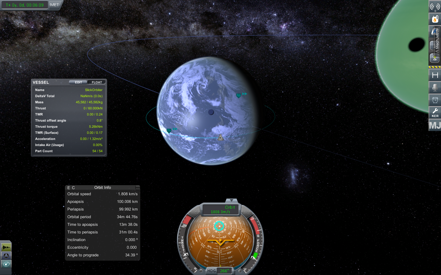
Given from what I have told you, you should be able to spot that it is a circular orbit (eccentricity = 0 or apoapsis \(\approx\) periapsis) and it’s orbital plane is perfectly aligned with the equatorial plane of the central body (inclination = 0).

Now you should be equipped with the basic toolset for the next post where we will be modifying orbital parameters with maneuvers.